


Data Structure and Algorithms (DSA) are two main computer science concepts that help to organize data efficiently. Data structure refers to the way the data is stored in the memory. The main idea behind data structures is to minimize time and space complexity. A good data structure is one which requires minimum storage and executes the process in minimum time. Algorithms are a group of instructions or steps to complete a task efficiently.
If you want to explore competitive programming further, a well profound knowledge of DSA is required.
Here is a glimpse of the data structures and the algorithms taken to get the desired output.
ARRAYS
An array is a linear data structure. It is a collection of similar data types where the data is stored in contiguous memory, allowing fast and efficient access. Here each element has an identified index. It is a fixed data structure where once the size is decided we cannot change it afterwards.
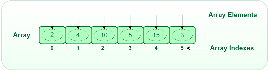
Arrays store elements of any data type like integer, character, string, float, etc. In most programming languages, arrays are zero-indexed i.e. the first element is at position zero, the second element at one, and so on. It also helps in implementing dynamic data structures like stack and queue. Here are a few available resources linked below to study the most basic topics of an array.
Reverse An Array - shifting the array in such a manner that the first element becomes the last element, the second element becomes the second last, and so on.
Multidimensional Array - forming matrix is the most common 2D array.
Linear Search - used to search an element in an array sequentially.
Binary Search - used in a sorted array by repeatedly dividing the search interval in half.
Subarray Sum - it prints the sum of all the possible subsequences of the given array.
BASIC SORTING ALGORITHMS
These algorithms arrange the elements in a certain order such as ascending or descending. They rearrange the elements of an array, list, or other data structure in order to make it easier to search, process or analyze data. Some of the most common sorting algorithms are:
Bubble Sort - This is a simple sorting algorithm that repeatedly steps through the list, compares adjacent elements, and swaps them if they are in the wrong order.
Selection Sort - This is an algorithm that works by dividing the input list into two parts: the sorted part at the left end and the unsorted part at the right end.
Insertion Sort - This is an algorithm that builds the final sorted array one item at a time.
Counting Sort - Counting Sort is a linear sorting algorithm that sorts elements based on the frequency of their values.
DIVIDE & CONQUER
Divide & conquer is a technique that involves breaking down a large, complex problem into smaller subproblems, solving each subproblem individually, and then combining the solution to the subproblems to get the solution of the original problem. The following techniques use the divide & conquer approach:
Quick Sort - It works by selecting a pivot element from the list and partitioning the other elements into two sublists, according to whether they are less than or greater than the pivot.
Merge Sort - Merge Sort is a divide-and-conquer sorting algorithm that sorts an array by dividing it into two halves, sorting each half, and then merging the two sorted halves back into one sorted array.
ARRAYLISTS
An ArrayList is a resizeable class in java in the java.util package. The main difference between array and ArrayList is the size of an array is fixed and can't be modified. While in ArrayList you can easily modify its size whenever you want. There are various operations that you can perform on an ArrayList:
Adding Elements - In order to add elements in an ArrayList, we use the add() method.
Changing Elements - to change the elements after adding, we can use the set() method.
Removing Elements - to remove an element from an ArrayList we use the remove() method.
Reverse the ArrayList - we can reverse the elements of the ArrayList.
LINKED LIST
A linked list is a linear data structure where the elements are not stored at contiguous memory locations. The elements are linked together using pointers.
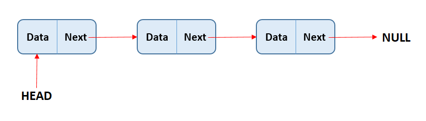
Each node has a data and the next pointer through which it is connected to the next node as shown in the picture above.
Here is a short description of each type of Linked List.
Types of linked lists:
Singly Linked List - A single linked list allows the traversal of the data in only one direction, going forwards as shown above. We can perform various operations like :
Insertion - We can add elements in the linked list.
Deletion - We can use it to delete the elements from the linked list.
Update - Used to update the contents of the LL.
Reverse the LL - The nodes of the LL are reversed, the first becomes the last one, the second becomes the second last and so on.
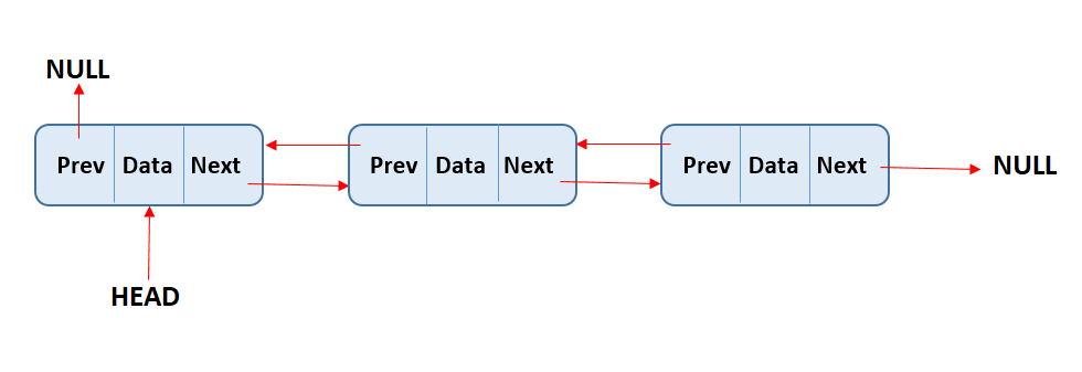
Doubly Linked List - A doubly linked list can be traversed in both forward and backward directions as shown below. It contains two pointers, a previous pointer that points to the data of the previous node. A next pointer that points to the data of the next node.We can perform the following operations on doubly LL:
Insertion - We can insert nodes in a doubly LL.
Deletion - To delete the nodes from the doubly LL.
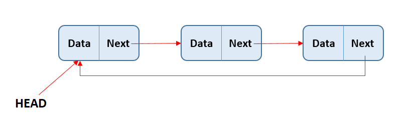
Circular Linked List - In circular linked list all the nodes are connected to each other in the form of a circle. The last node points to the first node of the linked list.
Insertion - to insert nodes in a circular LL.
Deletion - delete nodes from circular LL.
STACK
A stack is a linear data structure that follows the LIFO(Last In First Out) principle. This means the last item added to the stack will the first one to be removed. Imagine a stack of books, a deck of cards, etc.

We can perform many operations on a stack, the primary ones are:
push() - insert elements in a stack
pop() - delete elements from the stack.
peek() - to fetch the element on the top of the stack.
We can also implement stack using :
- Linked List - The stack is formed with the help of the linked list.
Stack using COLLECTIONS FRAMEWORK
Java Collections Framework is a group of classes and interfaces in the java standard library that provides collections of objects. We can easily create a stack using JCF. Here's the syntax:
Stack <Integer> s = new Stack<>(); //Integer data type
//s is the object
QUEUE
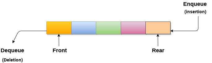
A queue is data structure where the elements can be inserted only at one end(rear) and deletion can only be done on the other end(front). This type of structure is known as the FIFO (First-In, First-Out) structure. We all have seen people standing in a queue when buying movie tickets or in the bank. These are some of the real-life examples of the queue.

We can easily add, delete elements in a queue. It is open from both sides, one side is the front-end(Dequeue) and the other is the rear-end(Enqueue).
You can follow the given resources to learn about the various operations in queue.
add() - inserts element in a queue.
remove() - removes the element at the front of the queue.
Queue using LL - we can implement a queue using Linked List.
Reverse a Queue - we can reverse the entire queue.
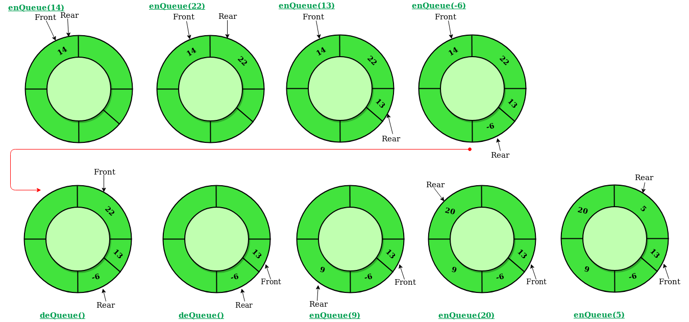
CIRCULAR QUEUE - A circular queue is a variation of the standard queue data structure with the added feature that when the end of the queue is reached, the next element is inserted at the beginning of the queue. This allows for efficient use of memory, as no space is wasted due to an empty region at the end of the queue.
BINARY TREES
A binary is a very important tree data structure in which each node has at most two child nodes, referred to as the left child and right child. The topmost node of the tree is called as the root node and the nodes which have no child nodes are called leaf nodes. This is how a binary tree looks:
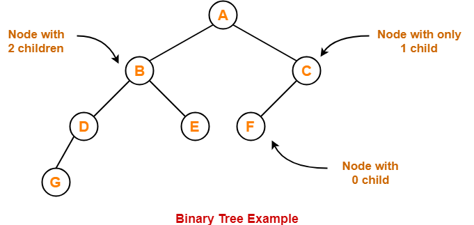
Here A is the root node. G, E, F are leaf nodes.
TREE TRAVERSALS - it is a process where we visit each node of the binary tree in any one of the three methods below:
Pre-Order Traversal - The nodes are visited in the order "Root-Left-Right".
Here's a function of Pre-order traversal code in Java:
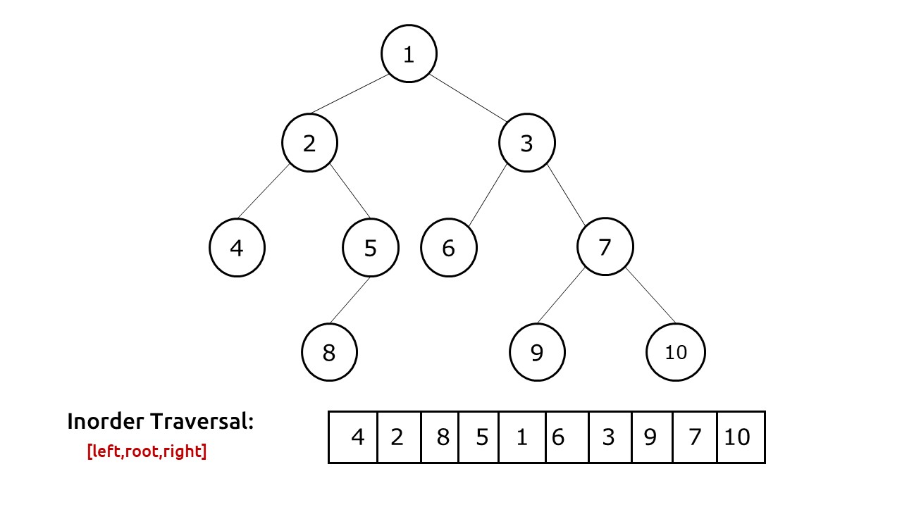
 public static void preorder(Node root) {
             if(root == null) {
                 return;
             }
             System.out.print(root.data + " ");
             preorder(root.left);
             preorder(root.right);
  }
In-Order Traversal - The nodes are visited in the order "Left-Root-Right".
Here's a function of In-order traversal code in Java:
 public static void inorder(Node root) {
             if(root == null) {
                 return;
             }
             inorder(root.left);
             System.out.print(root.data + " ");
             inorder(root.right);
 }

Post-Order Traversal - The nodes are visited in the order "Left-Right-Root".
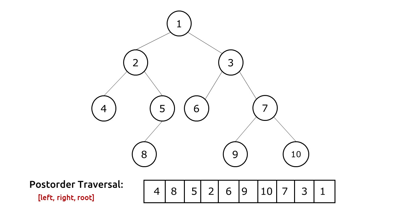
Here's a function of Post-order traversal code in Java:
public static void postorder(Node root) {
            if(root == null) {
                return;
            }
            postorder(root.left);
            postorder(root.right);
            System.out.print(root.data + " ");
}
Here are the links of the few important questions of binary trees:
Count Nodes - Count how many nodes are there in a binary tree.
Diameter of Tree - Diameter is the length of the longest path between two nodes of the binary tree.
Top View - print the top view of the binary tree.
Lowest Common Ancestor - LCA of two nodes is the deepest node which is the ancestor of both the nodes.
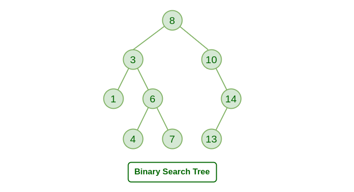
BINARY SEARCH TREE (BST)
A Binary Search Tree is a binary tree data structure where the values of the nodes of the left subtree are less than the value of the root node and the values of the right subtree are greater than the value of the root node. The left and right subtree each must also be a BST.
We can perform various operations on BSTs like:
Insert in BST - Inserting a node in BST.
Search in BST - We can search for a node in BST.
Delete in BST - De
lete a node from BST.
Print in Range - Print all the nodes lying between two keys, k1 and k2
Valid BST - to check if the given tree is BST or not.
Convert BST to balanced BST - converting the unbalanced tree into a balanced BST.
Merge two BSTs - merge two BSTs into one.
AVL TREE
An AVL Tree is a self balancing binary tree in which each node has a balanced factor which is either -1, 0, or 1 which is calculated by subtacting the height of its right subtree from that of its left subtree. The tree is said to be balanced if the balanced factor is -1, 0 or 1 otherwise it is considered unbalanced. The balancing process of an AVL tree is based on four rotations: left-rotation, right-rotation, left-right-rotation, and right-left-rotation. Each rotation is performed to maintain the balance of the tree and preserve its ordering properties.
For more reading links on AVL Trees, click here.
Red Black Tree
A red-black tree is a self-balancing binary search tree that is similar to AVL trees but with less stringent balancing requirements. The primary goal of a red-black tree is to ensure that the tree remains approximately balanced to ensure efficient operations.
In a red-black tree, each node is colored either red or black. The color of a node is used to ensure that the tree remains balanced. Specifically, the following properties must be satisfied:
Every node is either red or black.
The root is always black.
Every leaf (NULL) is black.
If a node is red, then both its children are black.
Every path from a node to any of its descendant leaves contains the same number of black nodes.
Refer to the link to read more.
HEAP
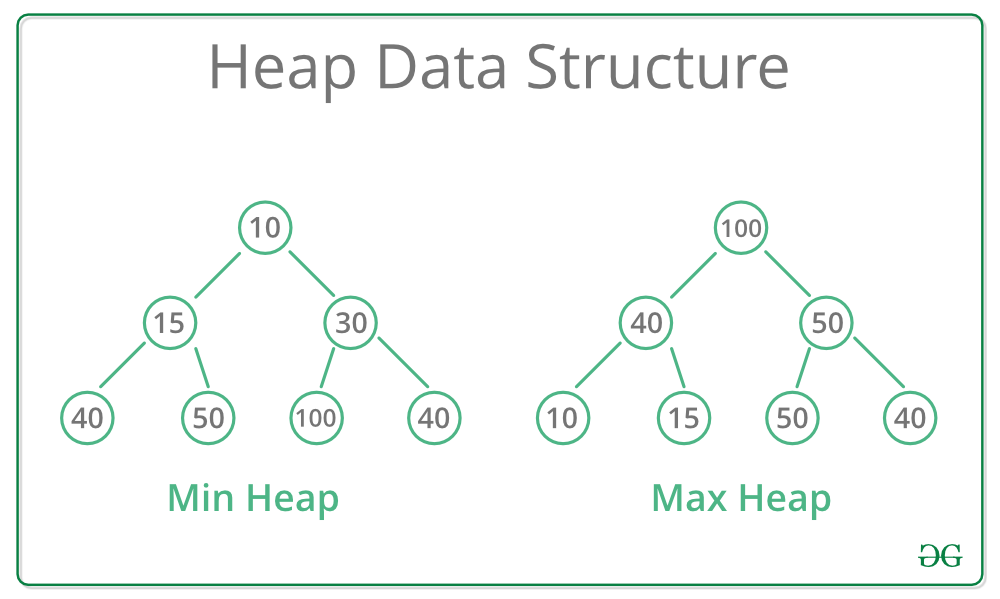
In computer science, a heap is a specialized tree-based data structure that satisfies the heap property. A heap is typically implemented as an array where elements can be thought of as nodes in a complete binary tree. The heap property defines the relationship between parent and child nodes.
There are two types of heaps: max heap and min heap. In a max heap, the value of each parent node is greater than or equal to the values of its children. In contrast, in a min heap, the value of each parent node is less than or equal to the values of its children.
Priority Queue
A priority queue is a data structure that allows efficient insertion and extraction of the highest (or lowest) priority element. It is similar to a regular queue in that it is a collection of elements that are ordered based on their arrival time, but it differs in that each element is also assigned a priority value.
Elements in a priority queue are stored based on their priority value, and the element with the highest priority is always at the front of the queue. When an element is removed from the priority queue, the element with the next highest priority takes its place.
We can easily the following operations on a heap:
insert and delete the elements from the heap. Click here.
Peek in heap - to retrieve or fetch the first element of the Queue.
Here's a question you can practice on leetcode : Sliding Window Maximum.
For more reading, click here.
HASHING
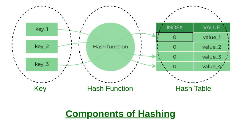
Hashing is a technique used in computer science to store and retrieve data quickly. It involves mapping data of arbitrary size to data of a fixed size, called a hash value, using a mathematical function called a hash function.
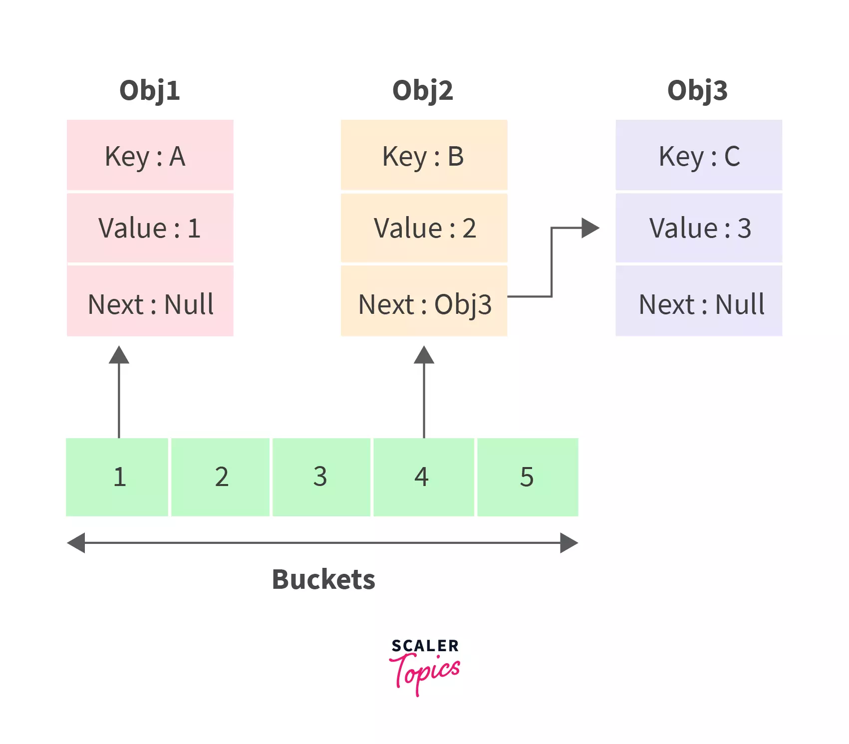
A hash function takes a key as input and outputs a hash value, which is a fixed-size representation of the key. The hash value is typically used as an index into an array, where the corresponding data is stored. The hash function should be designed to minimize the chance of collisions, which occur when two keys have the same hash value.
Java HashMap
Java HashMap class implements the Map interface which allows us to store key and value pair, where keys should be unique. If you try to insert the duplicate key, it will replace the element of the corresponding key. It is easy to perform operations using the key index like updation, deletion, etc. HashMap class is found in the java.util package.
HashMap Implementation Code:
 public boolean containsKey(K key) {
     int bi = hashfn(key);  // index of the bucket
     int di = getIndexWithinBucket(key,bi);  //index of the position in that
     //bucket
     if(di!=-1){  //if the di value is not equal to -1 return true, otherwise  //false
         return true;
     }
     else{
         return false;
     }
 }

 private int hashfn(K key){
     int hc = key.hashCode();
     return Math.abs(hc)%buckets.length;
 }

 private int getIndexWithinBucket(K key, int bi){
     int d1 = 0;
     for(Node node : buckets[bi]){
         if(node.key.equals(key)){
             return d1;
         }
         d1++;
     }
     return -1;
 }
Linked HashMap
A LinkedHashMap is a data structure in Java that combines the features of a hash table and a linked list. It maintains a doubly-linked list of the entries in the map, in the order in which they were inserted, and also provides constant-time performance for basic operations like get and put.
The LinkedHashMap class extends the HashMap class and provides the additional feature of maintaining the insertion order of the elements. This means that when you iterate over the entries of a LinkedHashMap, you get them in the same order in which they were added to the map.
In a LinkedHashMap, each entry in the map contains a reference to the next and previous entries in the linked list. This allows for efficient removal of elements from the map, as well as iteration over the entries in the map in insertion order.
For more reading, click here.
Tree Map
A TreeMap is a data structure in computer science that is used to store and manage a collection of key-value pairs in a sorted order based on the keys. It is implemented as a balanced binary search tree, which means that the tree is always balanced and the height of the tree is kept as small as possible. This ensures that the time complexity of basic operations, such as insert, search, and delete, is O(log n), where n is the number of elements in the TreeMap.
In a TreeMap, the keys are stored in a sorted order, which allows for efficient range queries and traversal of the key-value pairs in sorted order. TreeMap is similar to a HashMap, but it maintains the elements in sorted order based on the keys, rather than in the order in which they were inserted.
HashSet
HashSet is a data structure that is used to store a collection of unique elements, in which the order of the elements is not important. It is implemented as a hash table, which means that the elements are stored in an array and the index of the array is computed using a hash function.
One of the main advantages of using a HashSet is that it provides constant-time performance for basic operations such as add, remove, and contains, on average. This means that the time complexity of these operations is O(1), regardless of the size of the HashSet.
When adding an element to a HashSet, the element is hashed and the resulting hash code is used to compute the index of the array where the element should be stored. If there is no other element at that index, the element is simply stored there. If there is already an element at that index, the HashSet uses a collision resolution technique such as chaining or open addressing to handle the collision.
For more information, you can refer here.
Linked HashSet
LinkedHashSet is a data structure in Java that combines the features of a HashSet and a LinkedList. It is an implementation of the Set interface and maintains a doubly-linked list of the elements in the set, in the order in which they were inserted.
Similar to HashSet, LinkedHashSet stores a collection of unique elements in which the order is not important, and provides constant-time performance for basic operations such as add, remove, and contains. However, unlike HashSet, it maintains the insertion order of the elements.
The elements in a LinkedHashSet are stored in a hash table just like a HashSet, with the additional feature of maintaining a doubly-linked list to preserve the order of insertion. This means that the time complexity of basic operations is still O(1) on average, but iterating over the elements of a LinkedHashSet is guaranteed to be in the order of insertion.
TreeSet
TreeSet is a data structure in Java that implements the Set interface and stores a collection of elements in a sorted order. It is implemented as a self-balancing binary search tree, typically a Red-Black tree, which ensures that the time complexity of basic operations such as add, remove, and contains is O(log n), where n is the number of elements in the TreeSet.
One of the main advantages of using a TreeSet is that it provides efficient search and retrieval of the elements in the set in sorted order. This is useful when you need to maintain a sorted collection of elements and perform operations such as range queries or finding the smallest or largest element in the set.
Similar to other Set implementations, TreeSet stores a collection of unique elements in which the order is important. It does not allow duplicate elements, and the add() method returns false if the element is already in the set.
- You can practice the valid anagram problem here.
TRIES
It is a tree-like data structure that is commonly used for storing and retrieving strings in an efficient manner. A trie is also known as a prefix tree, because each node in the tree represents a prefix of one or more strings.
Each node in a trie represents a character, and each edge represents a transition to another node for the next character in the string. The root node represents an empty string, and each leaf node represents a complete string in the trie. For example, if we insert the strings "cat", "dog", "duck", and "dove" into a trie, the resulting trie would look like this:
           root
         /  |  \
        c   d   d
        |   |   |
        a   o   o
        |   |   | \
        t   g   v  u
                |   |
                k   e
You can perform operations like insert & search in a trie.
You can practice the following questions on tries:
GRAPHS
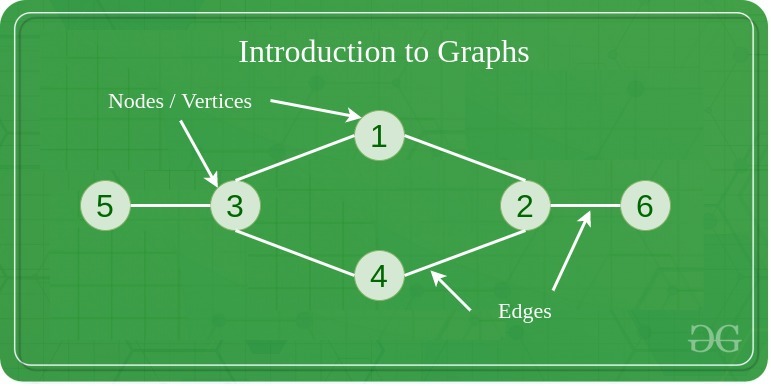
Graphs is the most important data structure in DSA. Most questions are asked from graphs. It is a non-linear data structure that consists of a set of vertices (also known as nodes) and a set of edges that connect pairs of vertices. Graphs are commonly used to model relationships and connections between objects in many real-world applications.
There are several types of graphs, including:
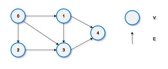
Directed graph or digraph: A graph in which each edge has a direction, meaning that the edges point from one vertex to another. In a directed graph, the edges are represented as arrows.
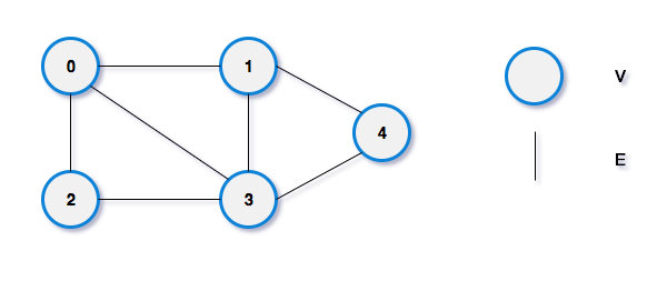
Undirected graph: A graph in which each edge has no direction, meaning that the edges do not point from one vertex to another. In an undirected graph, the edges are represented as lines.
Weighted graph: A graph in which each edge has a weight or cost associated with it. Weighted graphs are commonly used to model problems in which there are costs or distances associated with moving between vertices.

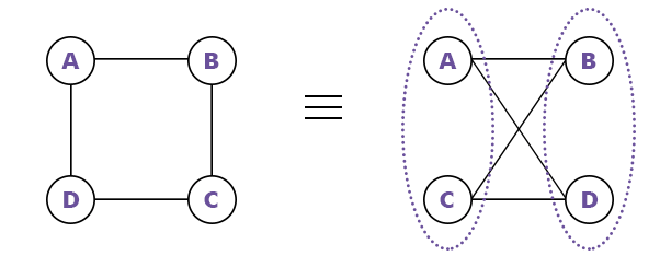
Bipartite graph: A graph in which the vertices can be divided into two disjoint sets, and every edge connects a vertex in one set to a vertex in the other set.
Here is an example of how you can create a graph data structure in Java using an adjacency list representation:
import java.util.*;

public class Graph {
    private int V;
    private LinkedList<Integer>[] adjList;

    public Graph(int v) {
        V = v;
        adjList = new LinkedList[v];
        for (int i = 0; i < v; i++) {
            adjList[i] = new LinkedList<>();
        }
    }

    public void addEdge(int u, int v) {
        adjList[u].add(v);
        adjList[v].add(u); // For undirected graph only
    }

    public void printGraph() {
        for (int i = 0; i < V; i++) {
            System.out.print(i + ": ");
            for (int j : adjList[i]) {
                System.out.print(j + " ");
            }
            System.out.println();
        }
    }

    public static void main(String[] args) {
        Graph g = new Graph(5);
        g.addEdge(0, 1);
        g.addEdge(0, 4);
        g.addEdge(1, 2);
        g.addEdge(1, 3);
        g.addEdge(1, 4);
        g.addEdge(2, 3);
        g.addEdge(3, 4);
        g.printGraph();
    }
}
In this example, we create a Graph class with an array of LinkedList objects to store the adjacency list for each vertex. The addEdge method is used to add an edge between two vertices, and the printGraph method is used to print the adjacency list for the graph.
In the main method, we create a new Graph object with 5 vertices and add some edges to the graph. Finally, we call the printGraph method to print the adjacency list of the graph.
BFS (Breadth First Search)
Breadth-first search (BFS) is a graph traversal algorithm that visits all the vertices in a graph in breadth-first order, i.e., it visits all the vertices at the same level before moving on to the vertices at the next level.
Here's an example of how to implement BFS in Java using an adjacency list representation of a graph:
import java.util.*;

public class BFS {
    private int V;
    private LinkedList<Integer>[] adjList;

    public BFS(int v) {
        V = v;
        adjList = new LinkedList[v];
        for (int i = 0; i < v; i++) {
            adjList[i] = new LinkedList<>();
        }
    }
    public void addEdge(int u, int v) {
        adjList[u].add(v);
        adjList[v].add(u); // For undirected graph only
    }
    public void BFS(int s) {
        boolean[] visited = new boolean[V];
        LinkedList<Integer> queue = new LinkedList<>();
        visited[s] = true;
        queue.add(s);

        while (queue.size() != 0) {
            s = queue.poll();
            System.out.print(s + " ");
            Iterator<Integer> it = adjList[s].listIterator();
            while (it.hasNext()) {
                int n = it.next();
                if (!visited[n]) {
                    visited[n] = true;
                    queue.add(n);
                }
            }
        }
    }
    public static void main(String[] args) {
        BFS g = new BFS(4);
        g.addEdge(0, 1);
        g.addEdge(0, 2);
        g.addEdge(1, 2);
        g.addEdge(2, 0);
        g.addEdge(2, 3);
        g.addEdge(3, 3);
        System.out.println("Following is Breadth First Traversal " +           "(starting from vertex 2)");
        g.BFS(2);
    }
}
We use a boolean array visited to keep track of the visited vertices and a LinkedList queue to keep track of the vertices that are yet to be visited. We start by marking the source vertex as visited and adding it to the queue. We then process each vertex in the queue by removing it from the front of the queue and visiting all its neighbors that have not been visited yet.
DFS (Depth First Search)
Depth-first search (DFS) is another popular graph traversal algorithm that visits all the vertices in a graph in depth-first order, i.e., it explores as far as possible along each branch before backtracking.
Here's an example of how to implement DFS in Java using an adjacency list representation of a graph:
import java.util.*;
public class DFS {
    private int V;
    private LinkedList<Integer>[] adjList;
    public DFS(int v) {
        V = v;
        adjList = new LinkedList[v];
        for (int i = 0; i < v; i++) {
            adjList[i] = new LinkedList<>();
        }
    }
    public void addEdge(int u, int v) {
        adjList[u].add(v);
        adjList[v].add(u); // For undirected graph only
    }
    public void DFSUtil(int v, boolean[] visited) {
        visited[v] = true;
        System.out.print(v + " ");
        Iterator<Integer> it = adjList[v].listIterator();
        while (it.hasNext()) {
            int n = it.next();
            if (!visited[n]) {
                DFSUtil(n, visited);
            }
        }
    }
    public void DFS(int v) {
        boolean[] visited = new boolean[V];
        DFSUtil(v, visited);
    }

    public static void main(String[] args) {
        DFS g = new DFS(4);
        g.addEdge(0, 1);
        g.addEdge(0, 2);
        g.addEdge(1, 2);
        g.addEdge(2, 0);
        g.addEdge(2, 3);
        g.addEdge(3, 3);

        System.out.println("Following is Depth First Traversal " + "(starting from vertex 2)");

        g.DFS(2);
    }
}
In this example, we create a DFS class with an array of LinkedList objects to store the adjacency list for each vertex. The addEdge method is used to add an edge between two vertices. The DFSUtil method is a helper method that takes a vertex and a boolean array visited as input and recursively visits all the vertices that can be reached from that vertex.
In the DFS method, we create a boolean array visited to keep track of the visited vertices and call the DFSUtil method to perform a DFS traversal starting from the input vertex.
In the main method, we create a new DFS object with 4 vertices and add some edges to the graph. Finally, we call the DFS method to perform a DFS traversal starting from vertex.
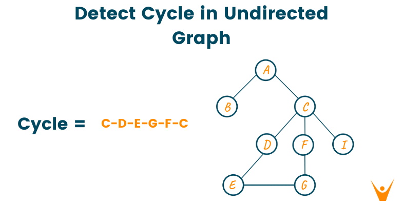
Cycle in Graph
A cycle in a graph is a path of vertices and edges that begins and ends at the same vertex. In other words, it is a closed path in the graph. Detecting cycles in a graph is an important problem in graph theory, and can be solved using various algorithms.
We can easily detect a cycle in:
Dijkstra's algorithm
Dijkstra's algorithm is a popular shortest path algorithm used to find the shortest path between two vertices in a weighted graph. It is a greedy algorithm that works by repeatedly selecting the vertex with the smallest distance from the source vertex and updating the distances of its neighboring vertices.
You can read in detail about the algorithm here.
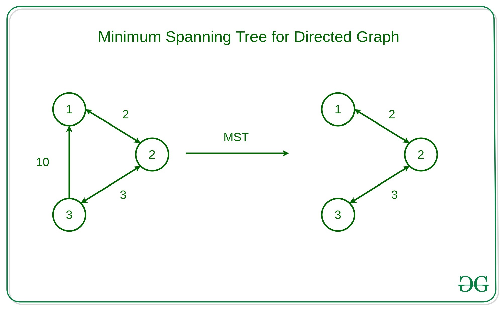
MST (Minimum Spanning Tree)
A minimum spanning tree (MST) of a connected, undirected graph is a tree that spans all the vertices in the graph with the minimum possible total edge weight. In other words, it is a subgraph that is both a tree (i.e., no cycles) and connects all the vertices of the graph. There are several algorithms to find the minimum spanning tree of a graph, with two popular ones being Prim's algorithm and Kruskal's algorithm.
Here's an example of how to implement PRIM'S ALGORITHM to find the minimum spanning tree of a weighted, undirected graph in Java:
import java.util.*;
public class PrimMST {
    private int V;
    private List<Edge>[] adjList;
    public PrimMST(int v) {
        V = v;
        adjList = new ArrayList[V];
        for (int i = 0; i < V; i++) {
            adjList[i] = new ArrayList<>();
        }
    }
    public void addEdge(int u, int v, int weight) {
        adjList[u].add(new Edge(v, weight));
        adjList[v].add(new Edge(u, weight)); // For undirected graph only
    }
    public void primMST(int source) {
        PriorityQueue<Node> pq = new PriorityQueue<>();
        boolean[] visited = new boolean[V];
        int[] parent = new int[V];
        int[] key = new int[V];
        Arrays.fill(key, Integer.MAX_VALUE);
        key[source] = 0;
        parent[source] = -1;
        pq.add(new Node(source, 0));
        while (!pq.isEmpty()) {
            int u = pq.remove().vertex;
            visited[u] = true;
            for (Edge e : adjList[u]) {
                int v = e.destination;
                int weight = e.weight;
                if (!visited[v] && weight < key[v]) {
                    key[v] = weight;
                    parent[v] = u;
                    pq.add(new Node(v, key[v]));
                }
            }
        }
        // Print the edges in the minimum spanning tree
        for (int i = 1; i < V; i++) {
            System.out.println("Edge " + parent[i] + " - " + i + " weight: " + key[i]);
        }
    }
    private static class Node implements Comparable<Node> {
        private int vertex;
        private int key;
        public Node(int vertex, int key) {
            this.vertex = vertex;
            this.key = key;
        }
        public int compareTo(Node other) {
            return Integer.compare(key, other.key);
        }
    }
    private static class Edge {
        private int destination;
        private int weight;
        public Edge(int destination, int weight) {
            this.destination = destination;
            this.weight = weight;
        }
    }

    public static void main(String[] args) {
        PrimMST g = new PrimMST(5);
        g.addEdge(0, 1, 2);
        g.addEdge(0, 3, 6);
        g.addEdge(1, 2, 3);
        g.addEdge(1, 3, 8);
        g.addEdge(1, 4, 5);
        g.addEdge(2, 4, 7);
        g.addEdge(3, 4, 9);
        g.primMST(0);
    }
}
Here's an example implementation of KRUSKAL'S ALGORITHM in Java. It works by initially sorting all the edges in the graph in non-decreasing order of their weights, and then iteratively adding the edges to the MST as long as they do not form a cycle.
import java.util.*;

public class KruskalMST {
    private int V, E;
    private Edge[] edges;
    public KruskalMST(int v, int e) {
        V = v;
        E = e;
        edges = new Edge[E];
    }
    public void addEdge(int index, int u, int v, int weight) {
        edges[index] = new Edge(u, v, weight);
    }
    public void kruskalMST() {
        Arrays.sort(edges);
        int[] parent = new int[V];
        for (int i = 0; i < V; i++) {
            parent[i] = i;
        }
        int count = 0;
        int index = 0;
        Edge[] mst = new Edge[V - 1];
        while (count < V - 1) {
            Edge e = edges[index++];
            int u = e.u;
            int v = e.v;
            int setU = find(parent, u);
            int setV = find(parent, v);
            if (setU != setV) {
                mst[count++] = e;
                parent[setU] = setV;
            }
        }
        // Print the edges in the minimum spanning tree
        for (int i = 0; i < V - 1; i++) {
            System.out.println("Edge " + mst[i].u + " - " + mst[i].v + " weight: " + mst[i].weight);
        }
    }
    private int find(int[] parent, int v) {
        if (parent[v] != v) {
            parent[v] = find(parent, parent[v]);
        }
        return parent[v];
    }
    private static class Edge implements Comparable<Edge> {
        private int u;
        private int v;
        private int weight;
        public Edge(int u, int v, int weight) {
            this.u = u;
            this.v = v;
            this.weight = weight;
        }
        public int compareTo(Edge other) {
            return Integer.compare(weight, other.weight);
        }
    }
    public static void main(String[] args) {
        KruskalMST g = new KruskalMST(5, 7);
        g.addEdge(0, 0, 1, 2);
        g.addEdge(1, 0, 3, 6);
        g.addEdge(2, 1, 2, 3);
        g.addEdge(3, 1, 3, 8);
        g.addEdge(4, 1, 4, 5);
        g.addEdge(5, 2, 4, 7);
        g.addEdge(6, 3, 4, 9);
        g.kruskalMST();
    }
}
The addEdge method is used to add an edge between two vertices with a given weight. The kruskalMST method is used to calculate the minimum spanning tree of the graph using Kruskal's algorithm.
- You can practice the Flood Fill problem here.
DYNAMIC PROGRAMMING
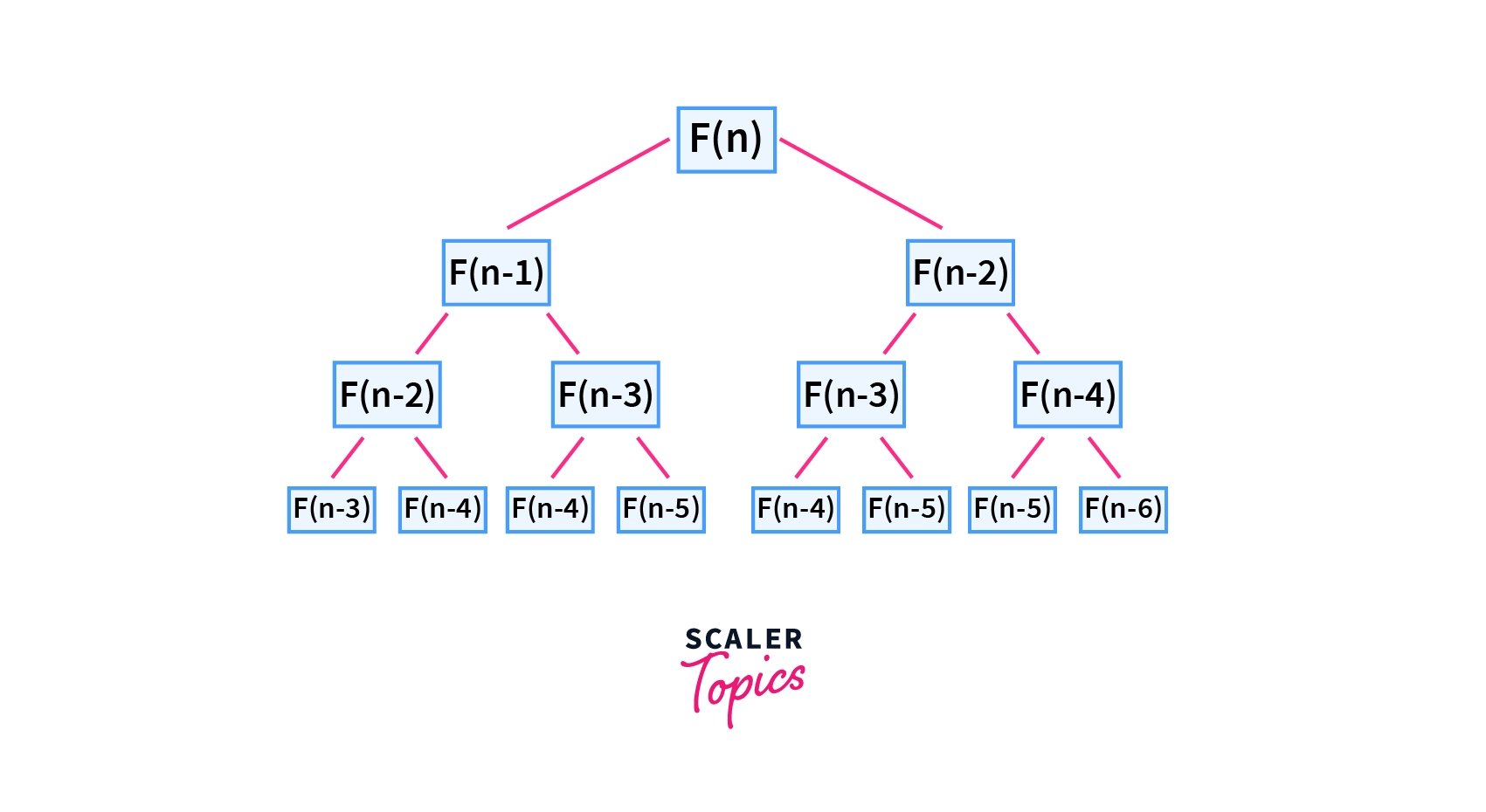
Dynamic programming is a technique used to solve complex problems by breaking them down into simpler subproblems and storing the results of these subproblems in memory so that they can be used to solve larger problems efficiently. Dynamic programming is based on the idea of overlapping subproblems, where the solutions to subproblems are reused multiple times.
There are two main types of dynamic programming: top-down and bottom-up. Top-down dynamic programming is also known as memoization, where we recursively solve subproblems and store the results in memory. Bottom-up dynamic programming, on the other hand, iteratively solves subproblems from the smallest subproblems up to the largest problem.
Here is an example of dynamic programming in Java that solves the famous Fibonacci sequence problem:
public static int fib(int n) {
    if (n == 0 || n == 1) {
        return n;
    }
    int[] memo = new int[n + 1];
    memo[0] = 0;
    memo[1] = 1;
    for (int i = 2; i <= n; i++) {
        memo[i] = memo[i - 1] + memo[i - 2];
    }
    return memo[n];
}
In this implementation, we calculate the nth Fibonacci number using a bottom-up approach. We first handle the base cases (n = 0 and n = 1), and then create an array memo to store the results of each subproblem. We then loop through each integer from 2 up to n, and store the sum of the previous two numbers in the memo array. Finally, we return the nth value in the memo array. This approach has a time complexity of O(n), as we only need to calculate each Fibonacci number once.
You can practice the classical problems of DP given below:
SEGMENT TREES
A segment tree is a data structure used to efficiently answer range queries on an array. It is commonly used for problems that involve finding the minimum, maximum, sum, or any other associative operation over a contiguous subarray of an array.
The basic idea behind a segment tree is to recursively divide the array into smaller subarrays, and store the results of the queries on each subarray in a binary tree. Each node in the binary tree represents a subarray, and stores the result of the query on that subarray. The root node of the tree represents the entire array.
To build a segment tree, we start with an array of n elements and build a binary tree where each leaf node represents a single element in the array. We then recursively compute the results for each parent node by combining the results of its children. For example, to compute the minimum value for a node, we can take the minimum of the minimum values of its two children.
Sum of given range in a segment tree.
Thus, with the help of this blog I've tried to write about each data structure in brief. To read in detail you can click on the links I've already provided. You can also practice the problems as they're frequently asked in interviews. Thank you for reading and I hope the blog was useful :):)