Time complexity is a measure of the amount of time required to run an algorithm or solve a problem as the input size grows larger. It is typically expressed in terms of the "Big O" notation, which gives an upper bound on the rate of growth of the running time as the input size increases.

Why efficient time complexity is important?

Efficient time complexity is important for several reasons. First, it can directly impact the user experience of an application. Users may become frustrated and abandon the application if an application takes too long to respond to user input or perform a task.

In addition, efficient time complexity can reduce the number of resources required to run a program. For example, if an algorithm has a time complexity of O(n^2), it will take much longer to solve a problem with a large input size than an algorithm with a time complexity of O(n). This can result in the need for more powerful hardware, which can be expensive and energy-intensive.

Overall, the efficient time complexity is desirable because it allows programs to handle larger and more complex tasks while minimizing the amount of time and resources required to complete them. This can improve applications' performance and scalability, making them more practical and useful for a wider range of use cases.

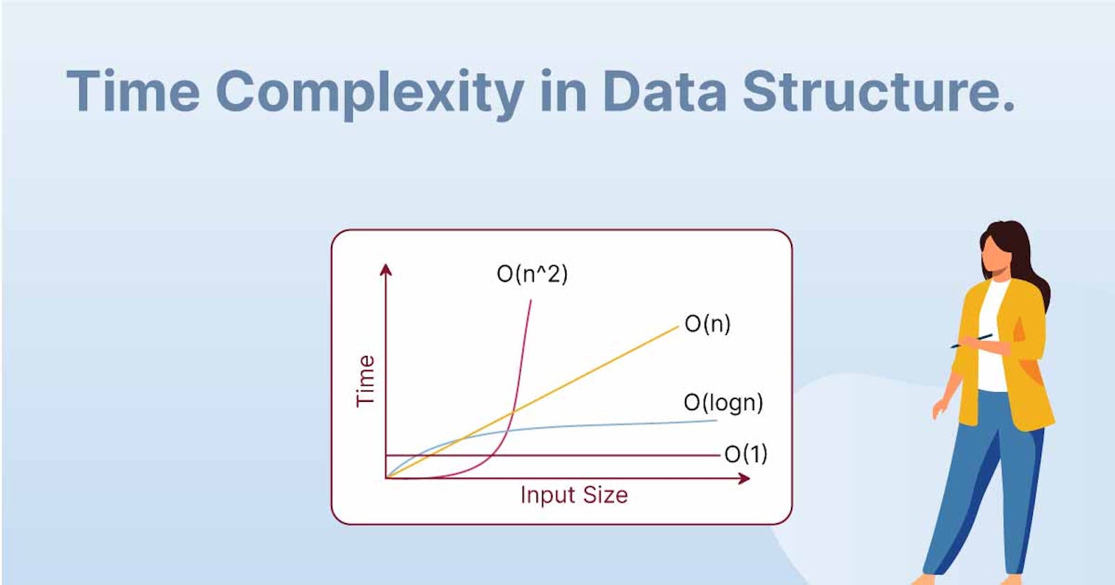
Asymptotic Notations

Asymptotic notations are used to describe the upper and/or lower bounds on the growth rate of an algorithm's time complexity as the input size grows larger. These notations are commonly used in computer science to analyze the efficiency of algorithms and compare different algorithms based on their performance.

1. Big-O Notation (O): This notation represents the upper bound of an algorithm's running time, which means it measures the worst-case time complexity or the longest amount of time an algorithm can take. For example, if the time complexity of an algorithm is O(n^2), it means that the algorithm's running time will not exceed n^2 for sufficiently large input sizes. Example: The worst-case time complexity of the Bubble Sort algorithm is O(n^2), where n is the number of elements in the input array. We generally consider this notation when we are asked to calculate time complexity.

2. Big-Omega Notation (Ω): This notation represents the lower bound of an algorithm's running time, which means it measures the best-case time complexity or the shortest amount of time an algorithm can take. For example, if the time complexity of an algorithm is Ω(n), it means that the algorithm's running time will not be less than n for sufficiently large input sizes. Example: The best-case time complexity of the Bubble Sort algorithm is Ω(n), which occurs when the input array is already sorted.

3. Big-Theta Notation (Θ): This notation represents the tight bound of an algorithm's running time, which means it measures the average-case time complexity or the time an algorithm takes when considering both the best and worst cases. For example, if the time complexity of an algorithm is Θ(n^2), it means that the algorithm's running time will be close to n^2 for sufficiently large input sizes. Example: The average-case time complexity of the Bubble Sort algorithm is Θ(n^2), where n is the number of elements in the input array.

How to calculate Time Complexity?

Calculating the time complexity of an algorithm involves analyzing the algorithm's code to determine how the running time of the algorithm changes according to the size of the input or the loops in the program. Here are the general key steps to keep in mind while calculating the time complexity of an algorithm:

1. Determine the input for the algorithm, and what variable(s) represent its size. This could be the number of elements in an array, the length of a string, the length of a stack/queue, etc.

2. Identify the basic operation(s) in the algorithm that is performed repeatedly, and that dominate the running time of the algorithm. These are usually things like comparisons, assignments, or arithmetic operations.

3. Count the number of times that each basic operation is executed as a function of the input size. For example, if there is a loop that runs n times and performs one comparison each time, then the total number of comparisons would be n.

4. Use the counts from step 3 to express the running time of the algorithm as a function of the input size. For example, if an algorithm has a loop that performs n comparisons, the running time could be expressed as T(n) = n.

5. Ignore the constants: Simplify the function from step 4 by removing constant factors and lower-order terms, and identifying the dominant term. This will give you the time complexity of the algorithm. For example, if the function from step 4 is T(n) = 5n + 3, the simplified function would be T(n) = O(n), because the constant factor (5) and the lower-order term (3) are both negligible compared to the dominant term (n).

At first, it may seem a bit confusing but with time and practice calculating the time complexity becomes easier.

Identifying Time Complexity

1. Single for loop: For a single for loop which is iterating 'n' times, the time complexity is O(n).

    for(int i=0; i<n; i++) {
        System.out.println("Hello World!");
    }
   

2. Nested for loop: In a nested for loop, since both the loops are iterating 'n' times, the time complexity will be multiplied, therefore it would be O(n^2).

    for(int i=0; i<n; i++) {
        for(int i=0; i<n; i++) {
            System.out.println("Hello World!");
        }
    }
   

3. Two individual for loops: In this, since both the loops are iterating independently 'n' and 'm' times, the time complexity will be added, therefore it would be O(n + m).

    for(int i=0; i<n; i++) {
        System.out.println("Hello");
    }
    for(int i=0; i<m; i++) {
        System.out.println("World!");
    }
   

Time Complexity of a few Algorithms and Data Structures

1. Insertion Sort

   The best time complexity is O(n) where n is the number of elements in the array. This occurs when the array is already sorted, and the algorithm only needs to make one pass over the array without swapping any elements.

   The worst-case time complexity of Insertion Sort is O(n^2), where n is the number of elements in the array. This occurs when the array is sorted in reverse order, and the algorithm needs to perform the maximum number of comparisons and swaps for each element in the array.

2. Bubble Sort

   The best-case time complexity of bubble sort occurs when the array is already sorted, in which case the algorithm would require only one pass to check that the array is sorted and no swaps would be needed. Thus, the best-case time complexity of bubble sort is O(n).

   The worst-case time complexity of bubble sort occurs when the array is in reverse order, and each element needs to be compared and swapped with every other element in the array to sort it. In this case, the worst-case time complexity of bubble sort is O(n^2).

3. Selection Sort

   The best-case time complexity of the selection sort is the same as the worst-case and the average-case time complexity, which is O(n^2).

4. Merge Sort

   The best-case scenario occurs when the elements are already sorted in ascending order and the worst case occurs when the elements are in decreasing order. Thus, the best-case, worst-case, and average-case time complexity of the merge sort is O(n*log(n)).

5. Linked List

   Searching: The best-case and worst-case time complexity for searching an element in a linked list are O(1) and O(n), respectively. In the best case, the element to be searched is at the head of the linked list, and the search can be completed in constant time. In the worst case, the element to be searched is at the end of the linked list, and we need to traverse the entire list to find it, which takes O(n) time.

   Insertion and Deletion: The best-case and worst-case time complexity for insertion and deletion operations in a linked list depends on the position of the element being inserted or deleted. In the best case, the element is inserted or deleted at the head of the linked list, and the operation can be completed in O(1) time. In the worst case, the element is inserted or deleted at the end of the linked list, and we need to traverse the entire list to reach that position, which takes O(n) time.

6. Queue

   Enqueue Operation: The best-case and worst-case time complexity for enqueue operation in a queue is O(1). In both cases, the operation involves inserting an element at the rear end of the queue, which takes constant time.

   Dequeue Operation: The best-case and worst-case time complexity for dequeue operation in a queue is O(1). In both cases, the operation involves removing an element from the front end of the queue, which takes constant time.

   Peek Operation: The best-case and worst-case time complexity for peek operation in a queue is O(1). In both cases, the operation involves accessing the element at the front end of the queue, which takes constant time.

7. Stack

   Push Operation: The best-case and worst-case time complexity for the push operation in a stack is O(1). In both cases, the operation involves inserting an element at the top of the stack, which takes constant time.

   Pop Operation: The best-case and worst-case time complexity for the pop operation in a stack is O(1). In both cases, the operation involves removing an element from the top of the stack, which takes constant time.

   Peek Operation: The best-case and worst-case time complexity for the peek operation in a stack is O(1). In both cases, the operation involves accessing the element at the top of the stack, which takes constant time.

8. Binary Tree

   Searching: The best-case and worst-case time complexity for searching an element in a binary tree is O(1) and O(h), respectively, where h is the height of the tree. In the best case, the element to be searched is at the root of the tree, and the search can be completed in constant time. In the worst case, the element to be searched is at the leaf of the tree, and we need to traverse the entire height of the tree to find it, which takes O(h) time.

   Insertion and Deletion: The best-case and worst-case time complexity for insertion and deletion operations in a binary tree also depends on the position of the element being inserted or deleted. In the best case, the element is inserted or deleted at the root of the tree, and the operation can be completed in O(1) time. In the worst case, the element is being inserted or deleted at the bottom-most level of the tree, and we need to traverse the entire height of the tree to reach that position, which takes O(h) time.

9. Graphs

   The time complexity of graphs also depends on the operation being performed and the type of graph.

   a. Searching: The best-case and worst-case time complexity for searching an element in a graph is O(1) and O(V+E), respectively, where V is the number of vertices and E is the number of edges in the graph. In the best case, the element to be searched is at the first vertex or edge visited, and the search can be completed in constant time. In the worst case, we need to traverse all vertices and edges in the graph to find the element, which takes O(V+E) time.

   b. Insertion and Deletion: The best-case and worst-case time complexity for insertion and deletion operations in a graph also depends on the position of the element being inserted or deleted. In the best case, the element is being inserted or deleted at the beginning of the adjacency list of a vertex, and the operation can be completed in O(1) time. In the worst case, we need to update the adjacency lists of all vertices and edges in the graph, which takes O(V+E) time.

   c. Shortest Path Algorithms: The time complexity of the Dijkstra's algorithm, which is used to find the shortest path between two vertices in a weighted graph, is O((V+E) log V) using a min-priority queue. The time complexity of the Bellman-Ford algorithm, which is used to find the shortest path in a graph with negative weights, is O(VE).

   d. Minimum Spanning Tree Algorithms: The time complexity of the Kruskal's algorithm and Prim's algorithm, which are used to find the minimum spanning tree of a weighted graph, are both O(E log E) or O(E log V), depending on the implementation.

So I hope you were able to understand the concept of time complexity a little bit better. For any doubts or queries, you can contact me anytime. I hope the blog was useful. Thank you for reading :)